| pol_b |
Political Ideology |
1. [1] extremely liberal
2. [2] liberal
3. [3] somewhat liberal
4. [4] moderate/middle of th
5. [5] somewhat conservative
6. [6] conservative
7. [7] extremely conservativ |
106 ( 7.9%)
173 (12.9%)
129 ( 9.6%)
474 (35.4%)
158 (11.8%)
173 (12.9%)
125 ( 9.3%) |
 |
1338
(91.3%) |
| pol_mod_b |
Liberal or Conservative |
1. [1] Liberal
2. [2] Conservative |
224 (47.5%)
248 (52.5%) |
|
472
(32.2%) |
| pol_party_b |
Party Affilitation |
1. [1] Strong Democrat
2. [2] Democrat
3. [3] Independent, leaning
4. [4] Independent
5. [5] Independent, leaning
6. [6] Republican
7. [7] Strong Republican |
162 (12.1%)
229 (17.2%)
157 (11.8%)
311 (23.3%)
140 (10.5%)
190 (14.2%)
145 (10.9%) |
|
1334
(91.1%) |
| pol_inde_b |
Democrat or Republican |
1. [1] Democrat
2. [2] Republican |
152 (49.7%)
154 (50.3%) |
|
306
(20.9%) |
| conservative |
Political Ideology |
1. [1] extremely liberal
2. [2] liberal
3. [3] somewhat liberal
4. [4] moderate/middle of th
5. [5] somewhat conservative
6. [6] conservative
7. [7] extremely conservativ |
106 ( 7.9%)
173 (12.9%)
129 ( 9.6%)
474 (35.4%)
158 (11.8%)
173 (12.9%)
125 ( 9.3%) |
|
1338
(91.3%) |
| conservative_bin |
|
Min : 0
Mean : 0.5
Max : 1 |
0 : 632 (47.3%)
1 : 704 (52.7%) |
|
1336
(91.2%) |
| republican_b |
|
Min : 0
Mean : 0.5
Max : 1 |
0 : 700 (52.7%)
1 : 629 (47.3%) |
|
1329
(90.7%) |
| conservative_f |
|
1. Liberal
2. Conservative |
632 (47.3%)
704 (52.7%) |
|
1336
(91.2%) |
| republican_f |
|
1. Democrat
2. Republican |
700 (52.7%)
629 (47.3%) |
|
1329
(90.7%) |
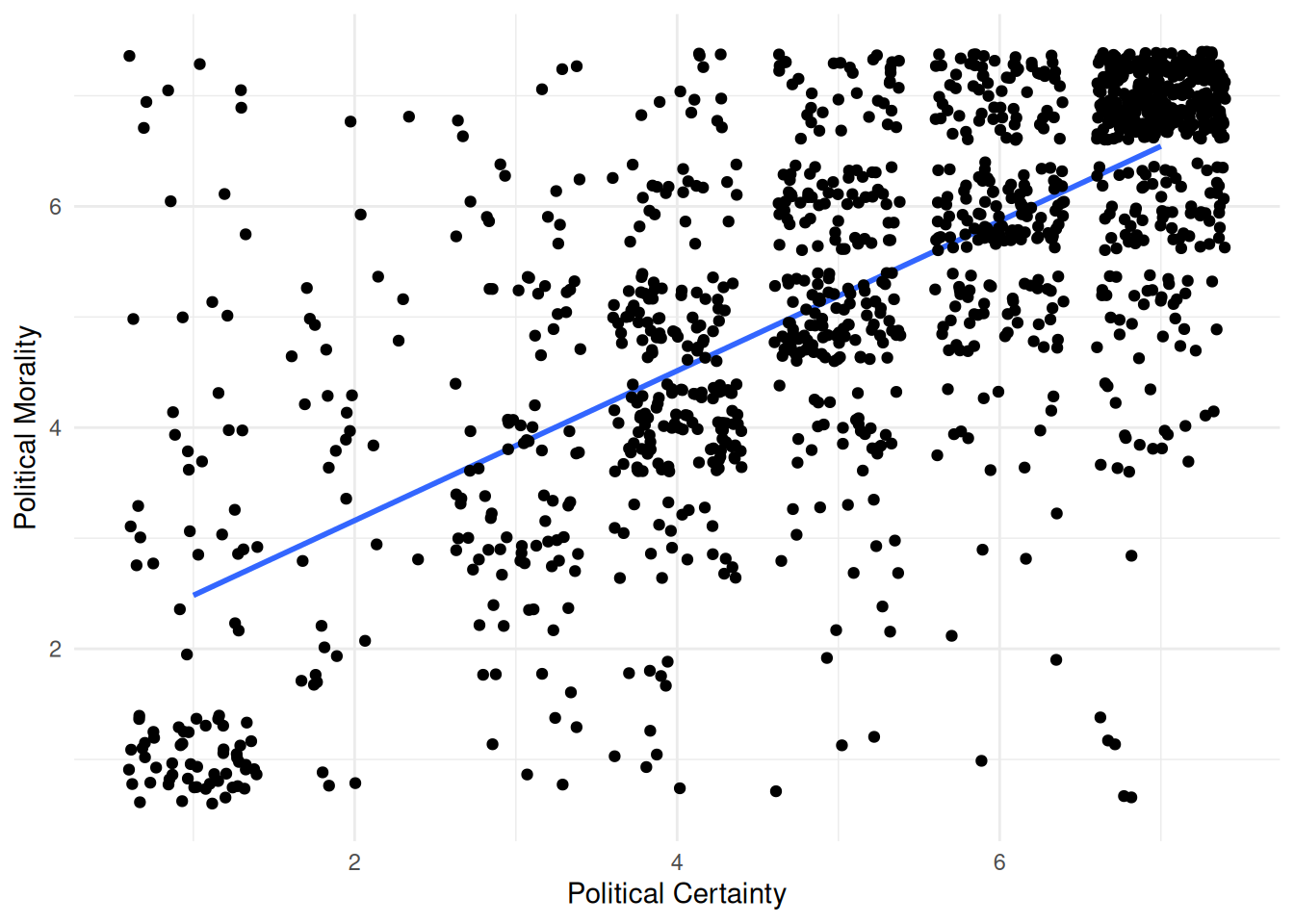
| polcert_b |
How certain are you in your political ideology? |
1. [1] 1
2. [2] 2
3. [3] 3
4. [4] 4
5. [5] 5
6. [6] 6
7. [7] 7 |
93 ( 7.0%)
35 ( 2.6%)
98 ( 7.3%)
212 (15.8%)
229 (17.1%)
225 (16.8%)
446 (33.3%) |
|
1338
(91.3%) |
| polmoral_b |
To what extent is your political ideology based in your core moral values? |
1. [1] 1
2. [2] 2
3. [3] 3
4. [4] 4
5. [5] 5
6. [6] 6
7. [7] 7 |
77 ( 5.8%)
34 ( 2.5%)
82 ( 6.1%)
181 (13.5%)
253 (18.9%)
255 (19.1%)
456 (34.1%) |
|
1338
(91.3%) |
| polStrength |
|
Mean (sd) : 5.2 (1.6)
min < med < max:
1 < 5.5 < 7
IQR (CV) : 2.5 (0.3) |
13 distinct values |
|
1338
(91.3%) |
| suppoppRep |
Are your political views motivated more by support for Republicans, or by opposition to Democrats? |
1. [1] 1 - not at all
2. [2] 2
3. [3] 3
4. [4] 4
5. [5] 5
6. [6] 6
7. [7] 7 - very much |
141 (22.6%)
69 (11.1%)
66 (10.6%)
233 (37.3%)
42 ( 6.7%)
23 ( 3.7%)
50 ( 8.0%) |
|
624
(42.6%) |
| suppoppDem |
Are your political views motivated more by support for Democrats, or by opposition to Republicans? |
1. [1] 1 - not at all
2. [2] 2
3. [3] 3
4. [4] 4
5. [5] 5
6. [6] 6
7. [7] 7 - very much |
161 (23.1%)
94 (13.5%)
81 (11.6%)
211 (30.2%)
73 (10.5%)
29 ( 4.2%)
49 ( 7.0%) |
|
698
(47.6%) |
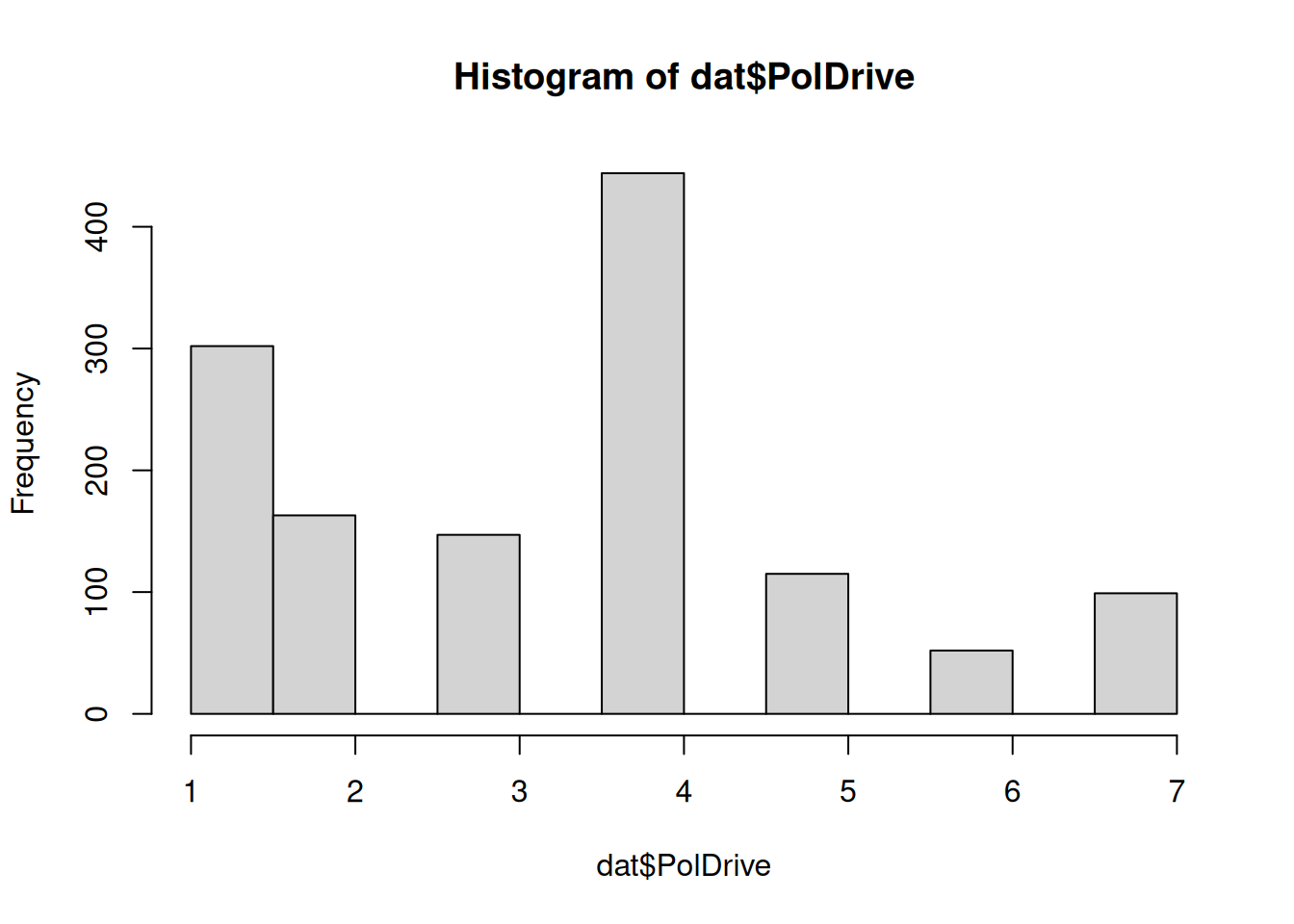
| PolDrive |
|
Mean (sd) : 3.3 (1.8)
min < med < max:
1 < 4 < 7
IQR (CV) : 2 (0.5) |
1 : 302 (22.8%)
2 : 163 (12.3%)
3 : 147 (11.1%)
4 : 444 (33.6%)
5 : 115 ( 8.7%)
6 : 52 ( 3.9%)
7 : 99 ( 7.5%) |
|
1322
(90.2%) |
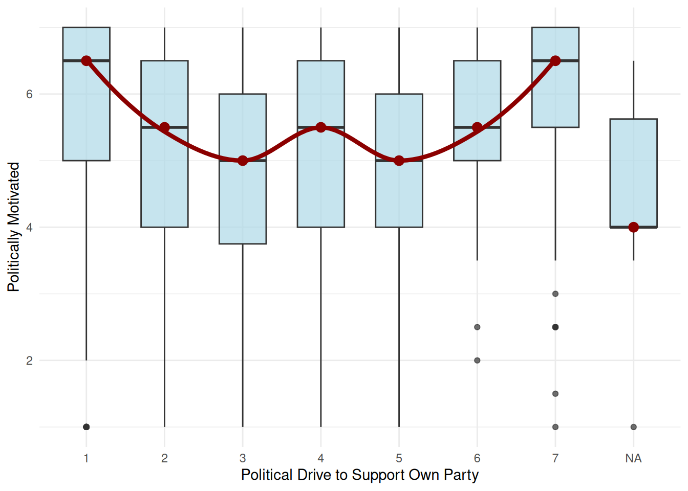
| polDrvSupOwnParty |
|
Mean (sd) : 3.3 (1.8)
min < med < max:
1 < 4 < 7
IQR (CV) : 2 (0.5) |
1 : 302 (22.8%)
2 : 163 (12.3%)
3 : 147 (11.1%)
4 : 444 (33.6%)
5 : 115 ( 8.7%)
6 : 52 ( 3.9%)
7 : 99 ( 7.5%) |
|
1322
(90.2%) |
| SelfInterBene1 |
In the long term, I appreciate considering a different perspective. |
1. [1] 1 - Strongly disagree
2. [2] 2 - Disagree
3. [3] 3 - Somewhat disagree
4. [4] 4 - Neither agree nor
5. [5] 5 - Somewhat agree
6. [6] 6 - Agree
7. [7] 7 - Strongly agree |
56 ( 4.3%)
47 ( 3.6%)
79 ( 6.1%)
368 (28.2%)
332 (25.5%)
241 (18.5%)
181 (13.9%) |
|
1304
(89.0%) |
| SIH2 |
I am willing to change my position on an important issue in the face of good reasons |
1. [1] 1 - Strongly Disagree
2. [2] 2
3. [3] 3
4. [4] 4
5. [5] 5
6. [6] 6
7. [7] 7
8. [8] 8
9. [9] 9 - Strongly Agree |
55 ( 4.2%)
27 ( 2.1%)
50 ( 3.8%)
112 ( 8.6%)
191 (14.7%)
172 (13.2%)
230 (17.7%)
194 (14.9%)
268 (20.6%) |
|
1299
(88.7%) |
| otherInterBene1 |
In the long term, other people in my political party appreciate considering a different perspective. |
1. [1] 1 - Strongly disagree
2. [2] 2 - Disagree
3. [3] 3 - Somewhat disagree
4. [4] 4 - Neither agree nor
5. [5] 5 - Somewhat agree
6. [6] 6 - Agree
7. [7] 7 - Strongly agree |
46 ( 3.5%)
70 ( 5.4%)
132 (10.1%)
509 (39.0%)
274 (21.0%)
154 (11.8%)
119 ( 9.1%) |
|
1304
(89.0%) |
| OtherSIH2 |
Other people in my political party are willing to change their positions on an important issue in the face of good reasons |
1. [1] 1 - Strongly Disagree
2. [2] 2
3. [3] 3
4. [4] 4
5. [5] 5
6. [6] 6
7. [7] 7
8. [8] 8
9. [9] 9 - Strongly Agree |
55 ( 4.2%)
45 ( 3.5%)
68 ( 5.2%)
167 (12.9%)
296 (22.8%)
192 (14.8%)
188 (14.5%)
134 (10.3%)
151 (11.7%) |
|
1296
(88.5%) |
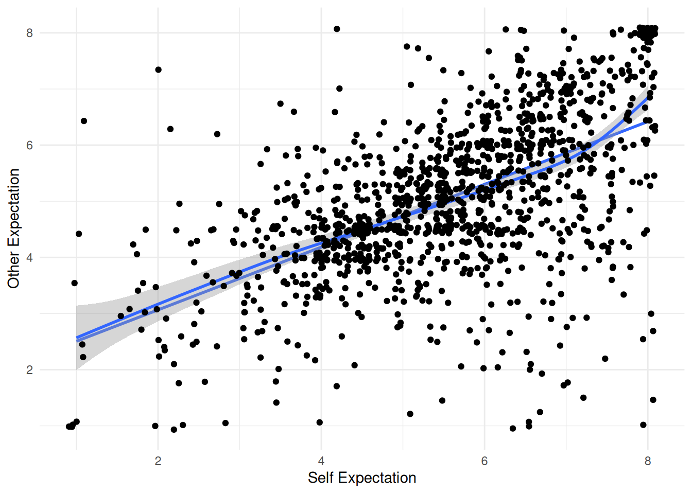
| selfTotal |
|
Mean (sd) : 5.6 (1.5)
min < med < max:
1 < 5.8 < 8
IQR (CV) : 2.2 (0.3) |
28 distinct values |
|
1299
(88.7%) |
| otherTotal |
|
Mean (sd) : 5.1 (1.4)
min < med < max:
1 < 5 < 8
IQR (CV) : 1.8 (0.3) |
29 distinct values |
|
1296
(88.5%) |
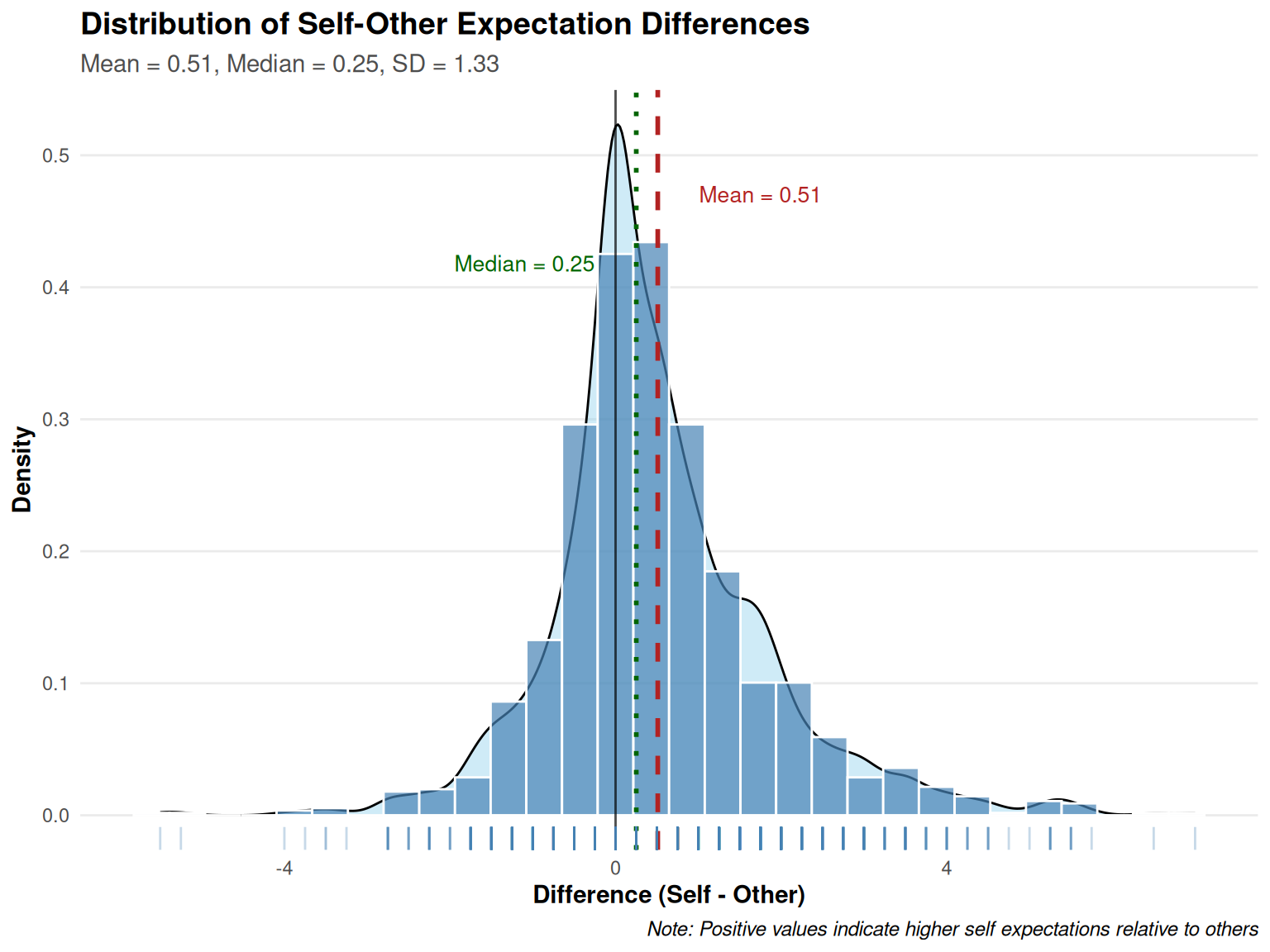
| ExpDelta |
|
Mean (sd) : 0.5 (1.3)
min < med < max:
-5.5 < 0.2 < 7
IQR (CV) : 1.2 (2.6) |
43 distinct values |
|
1293
(88.3%) |
| JE |
|
Mean (sd) : 4.5 (1.4)
min < med < max:
1 < 4.5 < 7
IQR (CV) : 1.5 (0.3) |
25 distinct values |
|
1242
(84.8%) |
| DS |
|
Mean (sd) : 3.4 (1.7)
min < med < max:
1 < 3.8 < 7
IQR (CV) : 2.5 (0.5) |
25 distinct values |
|
1242
(84.8%) |
| ST |
|
Mean (sd) : 3.4 (1.5)
min < med < max:
1 < 3.5 < 7
IQR (CV) : 2 (0.4) |
25 distinct values |
|
1242
(84.8%) |
| TS |
|
Mean (sd) : 3.5 (1.5)
min < med < max:
1 < 3.8 < 7
IQR (CV) : 2 (0.4) |
25 distinct values |
|
1242
(84.8%) |
| GSC |
|
Mean (sd) : 3.9 (1.6)
min < med < max:
1 < 4 < 7
IQR (CV) : 2 (0.4) |
25 distinct values |
|
1242
(84.8%) |
| CSC |
|
Mean (sd) : 3.8 (1.6)
min < med < max:
1 < 4 < 7
IQR (CV) : 2.5 (0.4) |
25 distinct values |
|
1242
(84.8%) |
| learn1 |
When discussing politics, I seek to understand where others are coming from. |
1. [1] 1 - Strongly disagree
2. [2] 2 - Disagree
3. [3] 3 - Somewhat disagree
4. [4] 4 - Neither agree nor
5. [5] 5 - Somewhat agree
6. [6] 6 - Agree
7. [7] 7 - Strongly agree |
52 ( 4.2%)
47 ( 3.8%)
66 ( 5.3%)
296 (23.9%)
367 (29.6%)
255 (20.6%)
155 (12.5%) |
|
1238
(84.5%) |
| learn2 |
When discussing politics, I want to learn more about why others believe the things they do. |
1. [1] 1 - Strongly disagree
2. [2] 2 - Disagree
3. [3] 3 - Somewhat disagree
4. [4] 4 - Neither agree nor
5. [5] 5 - Somewhat agree
6. [6] 6 - Agree
7. [7] 7 - Strongly agree |
56 ( 4.5%)
51 ( 4.1%)
79 ( 6.4%)
298 (24.1%)
324 (26.2%)
281 (22.7%)
149 (12.0%) |
|
1238
(84.5%) |
| Openness |
|
Mean (sd) : 4.8 (1.4)
min < med < max:
1 < 5 < 7
IQR (CV) : 2 (0.3) |
13 distinct values |
|
1238
(84.5%) |
| persuade1 |
When discussing politics, I seek to convince other people to take my position. |
1. [1] 1 - Strongly disagree
2. [2] 2 - Disagree
3. [3] 3 - Somewhat disagree
4. [4] 4 - Neither agree nor
5. [5] 5 - Somewhat agree
6. [6] 6 - Agree
7. [7] 7 - Strongly agree |
165 (13.3%)
149 (12.0%)
134 (10.8%)
370 (29.9%)
220 (17.8%)
117 ( 9.5%)
83 ( 6.7%) |
|
1238
(84.5%) |
| persuade2 |
When discussing politics, I want to show others how correct my opinion is. |
1. [1] 1 - Strongly disagree
2. [2] 2 - Disagree
3. [3] 3 - Somewhat disagree
4. [4] 4 - Neither agree nor
5. [5] 5 - Somewhat agree
6. [6] 6 - Agree
7. [7] 7 - Strongly agree |
153 (12.4%)
151 (12.2%)
123 ( 9.9%)
369 (29.8%)
221 (17.9%)
123 ( 9.9%)
98 ( 7.9%) |
|
1238
(84.5%) |
| persTot |
|
Mean (sd) : 3.9 (1.6)
min < med < max:
1 < 4 < 7
IQR (CV) : 2 (0.4) |
13 distinct values |
|
1238
(84.5%) |